CFA Note

CFA Level 3

Chapter: Capital Market Expectations (5-10%)

Trend Rate of Growth

$$\%\text{Growth}= \%\text{labor input} + \%\text{capital per worker} + \%\text{total factor productivity}$$

where:

• Labor input: labor force (population, demographics) + labor participation (real wages, work/leisure decision, social factors)
• capital per worker: increases labor productivity
• total factor productivity: technological progress + changes in government policies

Business Cycle Phases

The business cycle can be subdivided into five phases:

1. Initial Recovery

• Duration of a few months.
• Business confidence rising.
• Government stimulus provided by low interest rates and/or budget deficits.
• Decelerating inflation.
• Large output gap.
• Low or falling short-term interest rates.
• Bond yields bottoming out.
• Rising stock prices.
• Cyclical, riskier assets such as small-cap stocks and high yield bonds doing well.

2. Early Expansion

• Duration of a year to several years.
• Increasing growth with low inflation.
• Increasing confidence.
• Rising short-term interest rates.
• Output gap is narrowing.
• Stable or rising bond yields.
• Rising stock prices.

3. Late Expansion

• High confidence and employment.
• Output gap eliminated and economy at risk of overheating.
• Increasing inflation.
• Central bank limits the growth of the money supply.
• Rising short-term interest rates.
• Rising bond yields.
• Rising/peaking stock prices with increased risk and volatility.

4. Slowdown

• Duration of a few months to a year or longer.
• Declining confidence.
• Inflation still rising.
• Short-term interest rates at a peak.
• Bond yields peaking and possibly falling, resulting in rising bond prices.
• Possible inverting yield curve.
• Falling stock prices.

5. Contraction.

• Duration of 12 to 18 months.
• Declining confidence and profits.
• Increase in unemployment and bankruptcies.
• Inflation topping out.
• Falling short-term interest rates.
• Falling bond yields, rising prices.
• Stock prices increasing during the latter stages, anticipating the end of the recession.

Taylor rule

central bank uses taylor rule to make monetary policy decisions, determined by the target interest rate using the neutral rate, expected GDP relative to its long-term trend, and expected inflation relative to its targeted amount. It can be formalized as follows:

$$n_{target} = r_{neutral} + i_{expected} + \underbrace{[0.5(\text{GDP}_{expected} - \text{GDP}_{trend}) + 0.5(i_{expected} - i_{target})]}_{\text{adjustment}}$$

where:

• $n_{target}$ = target nominal short-term interest rate
• $r_{neutral}$ = neutral real short-term interest rate
• $\text{GDP}_{expected}$ = expected GDP growth rate
• $\text{GDP}_{trend}$ = long-term trend in the GDP growth rate
• $i_{expected}$ = expected inflation rate
• $i_{target}$ = target inflation rate

Macroeconomic linkage

A country’s current account and capital account are measures of macroeconomic linkages

$$\begin{aligned} \text{net exports} &= \text{net private saving} + \text{government surplus} \\ X - M &= (S - I) + (T - G) \end{aligned}$$

where:

• X = exports
• M = imports
• S = private savings
• I = investment spending
• T = tax
• G = government spending

GK Model

GK Model, i.e. Grinold-Kroner model, states that the expected return of a stock is its dividend yield, plus the inflation rate, plus the real earnings growth rate, minus the change in stock outstanding, plus changes in the P/E ratio:

$$\begin{aligned} E(R_e) & \approx \frac{D}{P} + \underbrace{(\%\Delta{E} - \%\Delta{S})}_{\text{growth rate of eps}} + \%\Delta{\frac{P}{E}} \\ & \approx \underbrace{\frac{D}{P} - \%\Delta{S}}_{\text{income (cash flow) return}} + \underbrace{\%\Delta{E}}_{\text{nominal earnings growth}} + \underbrace{\%\Delta{\frac{P}{E}}}_{\text{repricing return}} \\ & \approx \underbrace{\frac{D}{P} + g}_{\text{constant growth model}} + i - \%\Delta{S} + \%\Delta{\frac{P}{E}} \\ & \approx \frac{D}{P} + \underbrace{g + i}_{\text{Nominal GDP Growth}} && \text{(in the long run)} \end{aligned}$$

where:

• $E(R_e)$ = expected equity return
• $\frac{D}{P}$ = dividend yield
• $\%\Delta{E}$ = expected percentage change in total earnings
• $\%\Delta{S}$ = expected percentage change in shares outstanding, e.g. share repurchase means negative $\%\Delta{S}$, increasing $E(R_e)$
• $\%\Delta{P/E}$ = expected percentage change in the P/E ratio
• all the inputs should be forward-looking (i.e. forecast)

note:

• a share repurchase is a negative $\%\Delta{S}$ term, thus increasing $E(R_e)$
• a nominal earnings growth rate is used, thus incorporating effects of inflation explicitly
• limitation: assumption of infinite time horizon, ignoring investment horizon
• limitation: a $\%\Delta{E}$ larger than GDP growth is not plausible, because it implies a perpetually expanding economy

Real Estate Variation:

$$E(R_{re}) = \text{cap rate} + \text{NOI growth rate} - \%\Delta{\text{cap rate}}$$

ST Model

ST Model, i.e. Singer-Terhaar model, international CAPM

$$\begin{aligned} R_i &= R_f + \beta_{i, M} (R_M - R_f) && \text{(CAPM)} \\ RP_i &= \beta_{i, M} \times RP_M && (\because RP = R - R_f) \\ &= \rho_{i, M} \cdot \sigma_i \cdot \underbrace{(\frac{RP_M}{\sigma_M})}_{\text{Sharpe Ratio}} && (\because \beta_{i, M} = \rho_{i, M} \frac{\sigma_i}{\sigma_M}) \end{aligned}$$

Step1. Full integrated market

$$\begin{aligned} RP_i^G = \rho_{i, GM} \cdot \sigma_i \cdot (\frac{RP_{GM}}{\sigma_{GM}}) && (\text{+ e.g. liquidity premium}) \end{aligned}$$

Step2. Full segmented market

$$\begin{aligned} RP_i^S = \sigma_i \cdot (\frac{RP_{i}^S}{\sigma_{i}}) && (\text{+ e.g. liquidity premium}) \end{aligned}$$

Step3. weighted average risk premium

$$RP = \phi \cdot RP^G + (1 - \phi) \cdot RP^S$$

where:

• $\phi$ = degree of integration with the global markets

Step4. expected return

$$R = RP + R_f$$

Dornbusch overshooting mechanism

immediate capital flows will strengthen the currencies of countries with high expected returns to the point where the high return currency will be expected to depreciate going forward by the return differential.

$$\begin{aligned} E(\%\Delta S_{d/f}) &= (r^d - r^f) \\ &\quad + (\text{Term}^d - \text{Term}^f) \\ &\quad + (\text{Credit}^d - \text{Credit}^f) \\ &\quad + (\text{Equity}^d - \text{Equity}^f) \\ &\quad + (\text{Liquid}^d - \text{Liquid}^f) \end{aligned}$$

Chapter: Asset Allocation (5-10%)

MVO

MVO, i.e. Mean-variance optimization

$$max(\text{Utility}) = E(R) - 0.005 \times \lambda \times Var$$

where:

• $\lambda$ = risk aversion score

note:

• E® and Var are in % terms, if using decimal, times 0.5 instead of 0.005

limitation:

• GIGO: results sensitive to inputs, e.g. expected return, standard deviation, and correlation
• Concentrated asset class allocations: often results in a highly concentrated subset of asset classes, with zero allocation to others, causing lack of diversification of asset classes
• Skewness and kurtosis: only looks at expected return and variance, while in realty, there is significant skewness and kurtosis in actual returns
• Liquidity constraint: does not automatically incorporate liquidity constraints, often resulting in over-allocation to illiquid assets.

Black-Litterman Model

Black-Litterman model, starts with the “optimal” portfolio weights from the global market portfolio and derive the expected returns consistent with those weights. Then adjust these return estimates (called implied returns) to do a traditional MVO and derive optimal portfolio weights for our particular investor.

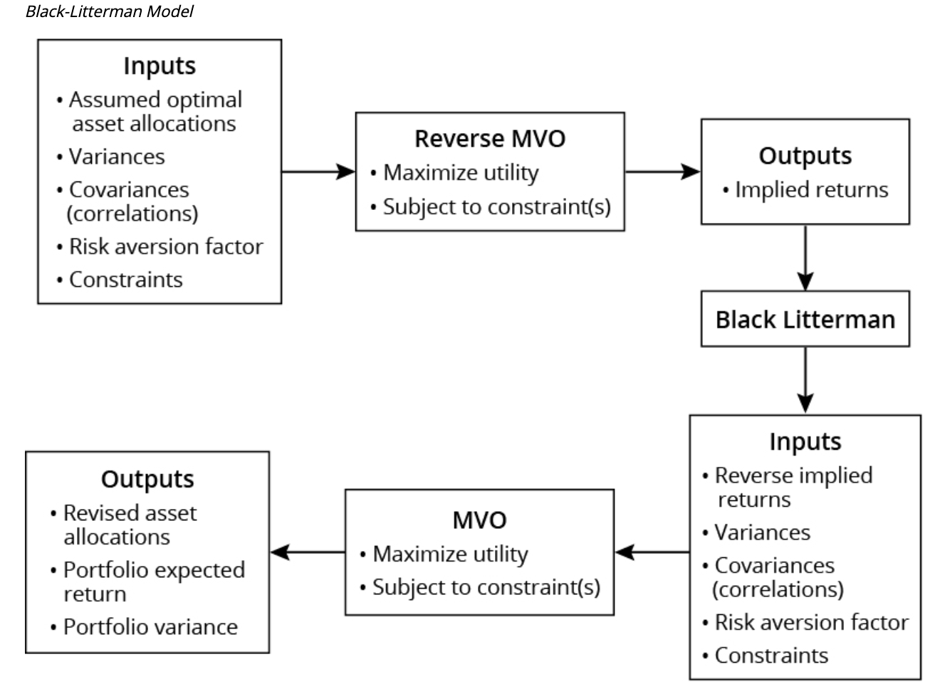
e.g.

• Derives an expected return for emerging market equities of 6.5% and you believe this is too low, you could adjust the expected return by 75 basis points to 7.25%. You can then rerun the MVO using your adjusted return estimates.
• Projects a return for U.K. large-cap equities of 8.2% and U.S. large-cap equities of 8.0% (a return differential of 20 basis points) and you believe that U.S. large-cap equities will outperform U.K. large-cap equities by 100 basis points, adjust the differential.

pros:

• world market weights are fully diversified and theoretically optimal
• less dependent on initial return estimates
• resulting portfolios are likely to contain more asset classes

Heuristic approach

60/40 rule

60% equity, 40% fixed income for the average individual

120 minus age

120 − age = % allocation to equities, with the remainder going to fixed incomes.

Risk budgeting approach

The goal of risk budgeting is to maximize return per unit of risk (e.g. total portfolio risk, active risk, or residual risk.)

$$\begin{aligned} \text{MCTR}_i &= \beta_{i, p} \times \sigma_p \\ \text{ACTR}_i &= w_i \times \text{MCTR}_i \end{aligned}$$

where:

• $\text{MCTR}_i$ = Marginal contribution to total risk, i.e. the change in total portfolio risk for a small change in the asset allocation to a specific asset class. i.e. the partial derivative of risk with respect to changes in portfolio allocations
• $\beta_{i, p}$ = beta of asset class i with respect to the portfolio
• $\sigma_p$ = total portfolio risk, i.e. standard deviation
• $\text{ACTR}_i$ = Absolute contribution to total risk, % of risk contributed by $\text{position}_i$= $\text{ACTR}_i$ / total portfolio risk

Chapter: Fixed Income

LDI types

Four types of liability-driven investing (i.e. LDI)

• Type I: Known future amount(s) and payout dates(s)
• Type II: Known future amount(s) but uncertain payout dates(s)
• Type III: Uncertain future amount(s) but known payout dates(s)
• Type IV: Uncertain future amount(s) and uncertain payout dates(s)

Immunization

Steps to compute Portfolio statistics:

1. Project the time to receipt (starting with the nearest to most distant) of every portfolio cash flow.
2. Determine the aggregate portfolio cash flow in each period. The analysis uses six-month periods.
3. Determine the portfolio IRR that equates future cash flows with the current market value of the portfolio.
4. Use that IRR to determine the PV of each future cash flow from Step 2. (The sum of those PVs will be the current portfolio market value.)
5. Calculate the PV weight (w) to apply to each payment as its PV (Step 4) divided by the sum of the PVs.
6. For each cash flow, multiply its (w) by its time until receipt(t). The sum of the (w)(t)s is the portfolio’s Macaulay duration. Duration is normally expressed in years, so if the cash flow periods were in six-month increments, divide by 2 (two six-month periods in a year) for annual duration.
7. Portfolio dispersion is computed as the weighted average variance of when each cash flow is received around portfolio duration. (Remember, duration is just the weighted average of when all the cash flows are received).
8. Portfolio convexity can be computed by summing for each cash flow: [(t)(t + 1)(w)] and then divide this sum by (1 + portfolio $IRR_{periodic}$)2.

note:

• Portfolio statistics should be used for ALM work rather than traditional weighted average calculations based on each bond. With flat yield curve, there’s no diff. In an upward-sloping yield curve, portfolio duration and cashflow yield (i.e. IRR) will be higher-than-average duration and YTM of the bonds because portfolio statistics reflect all cash flows (and return) to be received and the longer maturity bonds will impact the portfolio for a longer time.
• The goal of the immunized portfolio is to earn the initial portfolio IRR, not the average YTM of the bonds. Earning the IRR means the portfolio will grow to a sufficient FV to fund the liability.

$$\text{convexity} = \frac{\text{Macaulay duration}^2 + \text{Macaulay duration} + \text{dispersion}}{(1 + \text{periodic IRR})^2}$$

The dispersion and convexity will indicate the risk exposure of the immunization strategy to structural risk from shifts and twists in the yield curve.

Cash flow matching strategy

the safest approach, may allow accounting defeasance to legally set aside assets dedicated to meet the liability (both to be removed from the B/S)

bullet, barbell, Laddered portfolios (created by bonds directly or target-date bond ETFs)

Duration matching strategy

more flexible and generally practical approach to funding multiple liabilities.

for single liability:

• PVA >= PVL
• $MD_A$ = $MD_L$
• minimize Convexity

for multiple liabilities:

• PVA >= PVL
• $BPV_A = BPV_L$
• $C_A >= C_L$ slightly

Contingent immunization (CI)

a hybrid active/passive strategy. As long as a surplus is significant, the portfolio can be actively managed. if the strategy is unsuccessful, the surplus will shrink, and the portfolio must be immunized before the surplus declines below zero

Hedge Duration Gap between PVA and PVL

Consider an underfunded pension (i.e. DB plan) fund (i.e. PVA < PVL)

1. using future contract

$$N_f \text{ for 100\% hedge} = \frac{\overbrace{\text{BPV}_L - \text{BPV}_A}^{\text{BPV Gap} }}{\text{futures BPV}}$$

where:

• $\text{futures BPV} \approx \frac{\text{BPV}_{\text{CTD}}}{\text{CF}_{\text{CTD}}}$

2. using interest rate swaps

receive-fixed swap has positive (+) duration; pay-fixed swap has negative (-) duration

e.g. receive-fixed swap:

$$\text{net swap BPV} = \text{fixed-side BPV} - \text{floating-side BPV}$$

$$\text{NP} = \frac{\text{BPV Gap}}{\text{net swap BPV}}$$

3. using swaption

• to increase asset duration (i.e. $\text{BPV}_A$, closing duration gap), buy receiver swaption
• to decrease asset duration (i.e. $\text{BPV}_A$, widening duration gap), buy payer swaption

3*. using swaption collar

• buy a receiver swaption at lower strike (i.e. SFR: swap fixed rate)
• sell a payer swaption at higher strike (to reduce the initial premium cost outlay)

note:

• the payoff looks like a short risk reversal, with interest rate as X-axis

Example: choosing an optimal strategy

The choice of optimal strategy will depend on the manager’s view of interest rates. Consider the DB plan with a duration gap and a need to increase asset duration.

1. Enter a receive-fixed swap versus pay MRR.
2. Buy a receiver swaption.
3. Enter a zero-cost collar composed of buying the receiver swaption and selling a payer swaption.

Premium Cost	Cost
2.5% fixed-rate swap	None
2.3% receiver swaption	75 bp
3.3% payer swaption	75 bp

• The receive 2.5% SFR swap is optimal if the manager expects the new SFR will be at or below 2.5%.

  • This is equivalent to buying 2.5% fixed-rate bonds (financed by borrowing at MRR), increasing asset duration and BPV. The plan will benefit from the decline in rates.
  • Buying the 2.3% receiver swaption is suboptimal because there is an initial cost, and the 2.3% fixed rate received by the plan is lower.
  • The collar (buy the 2.3% receiver swaption; sell the 3.3% payer swaption) is suboptimal because the 2.3% fixed rate received by the plan is lower. The payer swaption buyer has no rational reason to exercise his right with the new SFR below 3.3%.

• The collar is optimal if the manager expects the new SFR will be above 2.5% but below 3.3%.

  • The collar (buy the 2.3% receiver swaption and sell the 3.3% payer swaption) has no intrinsic value, which is the best choice.
    • The right to receive 2.3% when rates are above 2.5% has no value.
    • The payer swaption buyer has no rational reason to exercise his right with new SFRs below 3.3%.
  • The other hedges have negative value or zero value with an up-front cost.
    • The swap of receive 2.5% will have negative value when SFRs are above 2.5%.
    • The receiver swaption (right to receive 2.3%) has no value when new SFRs are above 2.5% and required an initial cost.

• Buying the 2.3% receiver swaption is optimal at some level of new SFRs above 3.3%.

  • The 2.3% receiver swaption has no intrinsic value with new SFRs above 3.3%. But there was an initial premium cost. This is the best case at some level of SFRs above 3.3%.
  • The receive 2.5% swap has increasing negative value as new SFRs increase above 3.3%.
  • The collar also begins to have increasing negative value as new SFRs increase above 3.3%.
    • The receive 2.3% swaption has no value.
    • The 3.3% payer swaption increases in value as SFRs increase above 3.3%, and this is negative value to the seller (the plan).
    • As SFRs increase, that negative value will at some point exceed the initial cost of the receiver swaption, and the receiver swaption would become optimal.
    • The breakeven rate to make the payer swaption optimal is above 3.3%.

Fixed-income return decomposition

• 1. rolling yield:
  • a. coupon income = annual coupon amount / current bond price
  • b. rolldown return = (projected bond price (BP) assuming not yield curve change - beginning BP) / beginning BP
• 2. expected price change due to change in benchmark yield = $(-MD \times \Delta{Y}) + (1/2 \times C \times \Delta{Y}^2)$
• 3. expected price change due to change in credit spreads = $(-MD \times \Delta{S}) + (1/2 \times C \times \Delta{S}^2)$
• 4. expected currency G/L

Credit Spread Measures

Yield Spread

yield spread or benchmark spread := bond YTM - closest maturity on-the-run govt bond

g-spread

g-spread := bond YTM - interpolated YTM of the two adjacent maturity on-the-run govt bonds

i-spread

i-spread, interpolated spread := bond YTM - maturity interpolated swap fixed rate

asset swap spread

ASW := bond fixed coupon - maturity interpolated swap fixed rate

represents the spread that the bond is offering over the floating market reference rate (MRR) over its life (assuming the bond is trading close to par). Since the swap can swap fixed rate with MRR, buying the bond and payer swap can synthesize MRR + ASW return.

z-spread

z-spread, zero-volatility spread, takes into account the term structure of spot rates. It uses a trial-and-error calculation to determine a single spread that, when added to risk-free spot rates, discounts the bond’s future cash flows back to its current market value.

note: CDS Spread, where the protection buyer pays a standardized fixed coupon adjusted by an up-front payment/receipt to reflect the fair value of the protection, should in theory, be equal to the z-spread that is earned on the underlying bond, since both are essentially a risk premium paid to the party facing the credit risk of the bond. However, differences between the CDS spread and the z-spread can occur due to technical reasons, such as the underlying bond price trading away from par, accrued interest on the underlying bond, and idiosyncratic features of the CDS protection. The $\text{CDS basis} := \text{CDS spread} - \text{z-spread}$. This is a useful measure for those trading CDS contracts.

option adjusted spread

option adjusted spread, OAS, is the only spread measure appropriate for assessing the credit/liquidity risk of bonds with embedded options. It uses an assumption of interest rate volatility to build an interest rate tree of possible paths for forward risk-free interest rates. Future cash flows are adjusted for the optionality of the bond along each path (i.e., to reflect whether the option would be exercised). The OAS is then a trial-and-error calculation to determine a single spread that, when added to every node of the interest rate tree of risk-free rates, discounts the bond’s adjusted future cash flows back to its current market value. By adjusting the cash flows of the bond to reflect expected interest rate volatility, the uncertainty of the cash flows due to the optionality of the bond has been removed, and the resulting OAS, therefore, does not include any impact of the option on the spread. The OAS measures the spread that is earned for facing the credit and liquidity risk of the issuer—the impact of the option has been removed from the spread.

The OAS is the best measure for consistent comparison of the spreads on bonds with embedded options (e.g., callable, putable) and bonds without embedded options.

Excess Spread

excess spread: spread in excess of the fair spread for suffering credit losses.

$$\text{Excess Spread} := \text{Spread} - \text{EffSpreadDur} \times \Delta \text{Spread} - \underbrace{\text{POD} \times \text{LGD}}_{\text{credit loss, credit spread}}$$

Where:

• EffSpreadDur: Effective Spread Duration
• POD: Probability of Default
• LGD: Loss Given Default, i.e. loss severity, 1 - RR (recovery rate)
• Spread and POD should be de-annualized to match holding period, if given as annualized

note:

• Credit valuation adjustment (CVA), computed as the present value of sum of expected credit losses := POD * LGD for all periods scaled up by the expected exposure at the time of default. CVA represents the discount that the credit-risky instrument should trade below an equivalent risk-free security in order to compensate investors for their expected credit losses.

butterfly strategy

profit from a view that the curvature of the yield curve is likely to change, by combining long and short positions in bullets (i.e. body) and barbells (wings)

butterfly spread = - (short-term yield) + (2 x medium-term yield) - long-term yield

note:

• butterfly spread increase == curvature increase == negative butterfly twist == negative butterfly view (frowns more)

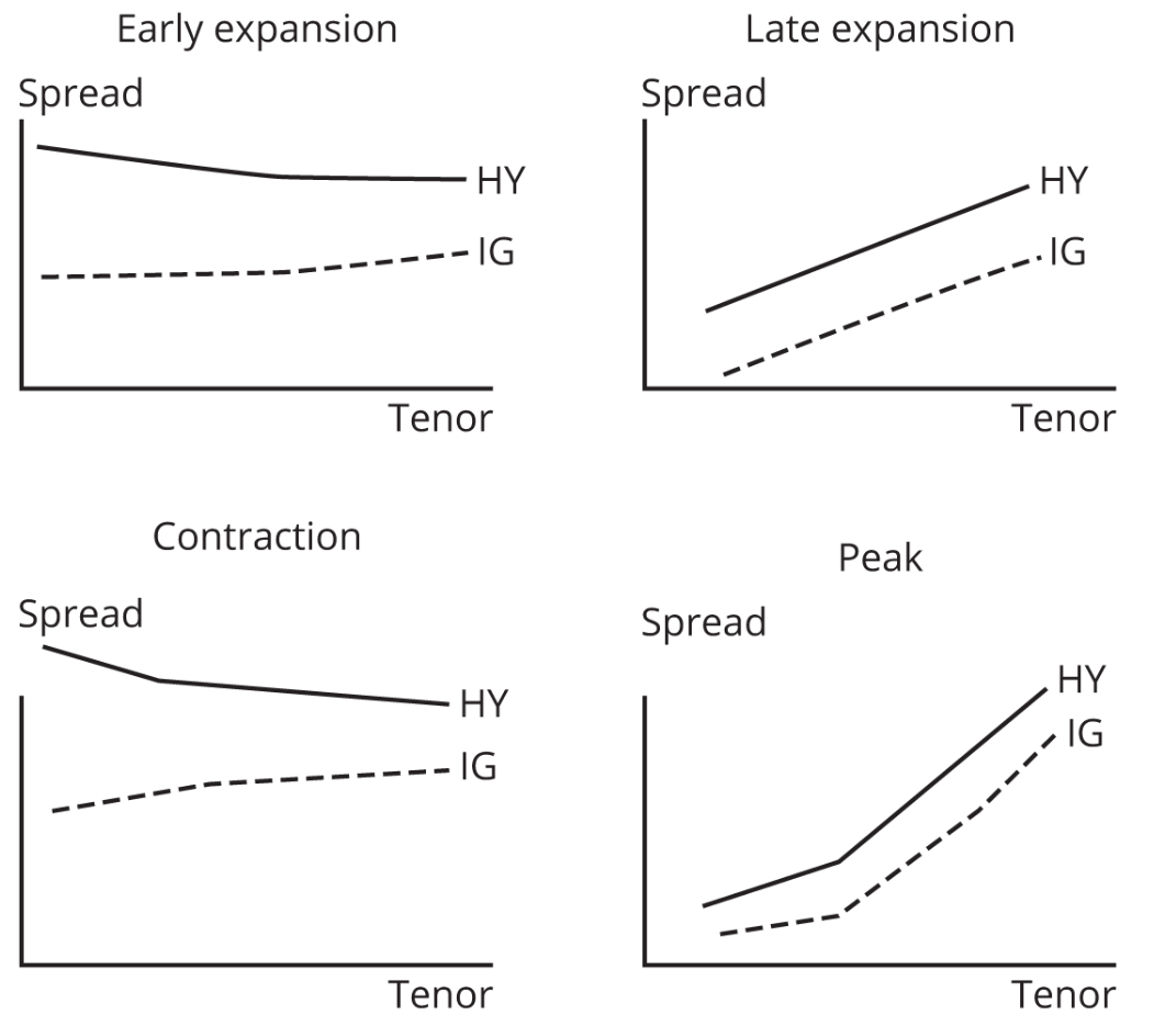
Credit Spread in Economic Cycle

	Early Expansion (Recovery)	Late Expansion	Peak	Contraction (Recession)
Corporate Defaults	Peak	Falling	Stable	Rising
Credit Spread Level	Stable	Falling	Rising	Peak
Credit Spread Slope IG	Stable	Upward sloping	Upward sloping	Flat
Credit Spread Slope HY	Inverted	Upward sloping	Upward sloping	Inverted
Corporate Leverage	Falling	Stable	Rising	Peak

CIRP

covered interest rate parity (i.e. CIRP) states that high interest rate currencies should trade at a forward discount

$$\text{forward rate}_{D/F} = \text{spot rate}_{D/F} \times \frac{(1 + r_D)^T}{(1+r_F)^T}$$

where:

• $\text{spot rate}_{D/F}$, $\text{forward rate}_{D/F}$: spot and forward rates denoted in direct quotes

Hedge Foreign Coupon-Paying Bonds

Consider an Australian investor who wishes to hedge their exposure to a coupon-paying U.S. Treasury bond. Assume current USD/AUD = 0.8

Position	At Initiation	Periodic Semiannual Payments for Next 10 Years	At the End
U.S. Treasury Bond	Pay out USD 100 million to purchase the U.S. bond	Receive-fixed USD bond coupon	Receive USD 100 million par at maturity of bond
Fixed-Fixed Cross-Currency Swap	Receive USD 100 million and pay AUD 125 million in exchange of principal amounts	Pay-fixed USD leg	Pay USD 100 million and receive AUD 125 million in exchange of principal amounts
Net Flow	Pay AUD 125 million principal outflow	Receive-fixed AUD payment	Receive AUD 125 million principal inflow

the fixed-fixed cross-currency swap can be synthesized by:

Swap	Description	Interest Paid	Interest Received	Principal Exchange at Outset	Principal Exchange at End
A	USD interest rate swap	USD Fixed	USD Floating	None	None
B	AUD interest rate swap	AUD Floating	AUD Fixed	None	None
C	Cross-currency basis swap	USD Floating	AUD Floating	Receive in USD principal, pay out AUD principal	Pay out USD principal, receive in AUD principal

Unhedged Cross-Currency Carry Trade

the carry trade involves borrowing in a low interest rate currency and depositing in a high interest rate currency, facing risk that high interest rate currency weakens.

total pnl = foreign returns - cost of funds + FX rate (D/F) return

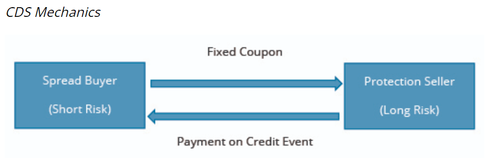
CDS

The protection buyer pays a regular fixed coupon to the protection seller periodically over the life of the contract in return for a payment upon a prespecified credit event on a reference issuer (or issuers). The size of the CDS is specified at the outset and referred to as the notional principal.

characteristics:

• OTC traded credit derivative
• Bilateral agreement
• Counterparty credit risk

The fixed coupon paid periodically by the protection buyer is standardized to 1% for investment-grade (IG) issuers and 5% for high-yield (HY) issuers for operational reasons, to make settlement and clearing of contracts more straightforward. Note this standardized coupon is not the fair premium that should be regularly paid by the protection buyer (referred to as the CDS spread) for the credit protection based on credit pricing models.

Scenario	Upfront Premium
CDS spread = fixed coupon	None
CDS spread > fixed coupon	[(CDS spread – fixed coupon) × EffSpreadDurCDS] paid to protection seller
CDS spread < fixed coupon	[(fixed coupon – CDS spread) × EffSpreadDurCDS] paid to protection buyer

CDS Price:

$$\text{CDS Price} ≈ 1 + (\text{Fixed Coupon} - \text{CDS Spread}) \times \text{EffSpreadDurCDS}$$

note:

• This pricing convention conforms with the usual inverse price/yield relationship seen in fixed income because, when CDS spreads rise, the CDS price will fall and vice versa.
• For higher-quality issuers, the CDS spread will be lower than the fixed coupon and the CDS price will be above par. For lower-quality issuers, the CDS spread will be higher than the fixed coupon and the CDS price will be below par.
• protection sell’s pnl is computed as [CDS price (t-1) - CDS price (t)] x Notional Principal

Position	Profit if CDS Spreads	Profit if CDS Prices
Sell protection (long risk)	Fall	Rise
Buy protection (short risk)	Rise	Fall

note:

• buy protection == long CDS spread == short risk == decrease exposure == short bond == short price

CDS long-short strategy

involves buying protection on issuers, where credit spreads are expected to widen relative to other issuers, while simultaneously selling protection on issuers, where credit spreads are expected to narrow relative to other issuers.

CDS curve trades

buying protection at maturities where CDS spreads are expected to rise relative to other maturities and selling protection at maturities where spreads are expected to fall relative to other maturities.

Credit Spread Curve Strategies

profit from a view on the shape or level of the credit spread curve.

Static Credit Spread Curve Strategies

A manager who believes that the current credit spread curve will remain unchanged can earn excess return in the cash market through either:

• lowering the average credit rating of their bond portfolio;
• increasing the spread duration by buying and holding longer-dated bonds.

Dynamic Credit Spread Curve Strategies

e.g. expect upward-sloping CDS curve to flatten, buy ST CDS protection, sell LT CDS protection

Economic Stage	Typical Curve Feature	Cash	CDS
Economic recovery	HY spreads narrow more than IG spreads	Buy HY bonds	Sell HY protection
		Sell IG bonds	Buy IG protection
	HY credit curve steepens	Buy short-term HY bonds	Sell short-term HY protection
		Sell long-term HY bonds	Buy long-term HY protection
Economic slowdown	HY spreads widen more than IG spreads	Buy IG bonds	Sell IG protection
		Sell HY bonds	Buy HY protection
	HY credit curve flattens/inverts	Buy long-term HY bonds	Sell long-term HY protection
		Sell short-term HY bonds	Buy short-term HY protection

Chapter: Equity

HHI

Herfindahl-Hirschman index (i.e. HHI):

$$\text{HHI} = \sum\limits_{i=1}^n{w_i^2}$$

$$\text{effective number of stocks} = \frac{1}{\text{HHI}}$$

where:

• n = the number of stocks in the portfolio
• ${w_i}$ = the weight of stock i

note:

• HHI ranges from 1/n (an equally-weighted portfolio) to 1 (a single stock portfolio)
• mcap-weighted portfolio has number of holdings larger than the number predicted by HHI, due to disproportionate effect of the largest capitalization stocks on the index

Decomposition of realized active return

realized (i.e. ex post) active return can be decomposed into:

$$R_A = \sum{(\beta_{pk} - \beta_{bk})} \times F_k + (\alpha + \epsilon)$$

where:

• $\beta_{pk}$ = the sensitivity of the portfolio to each rewarded factor (k)
• $\beta_{bk}$ = the sensitivity of the benchmark to each rewarded factor
• $F_k$ = the return of each rewarded factor
• ($\alpha + \epsilon$) = the return not explained by exposure to rewarded factors—alpha (α) is the active return attributable to manager skill, and ε is the idiosyncratic return—noise or luck (good or bad) (In practice it is very difficult to distinguish between α and ε)

Active Share

$$\text{Active Share} = \frac{1}{2}\sum\limits_{i=1}^n{|w_{p,i} - w_{b,i}|}$$

where:

• n = total number of securities in the benchmark or the portfolio
• $w_{p,i}$ = weight of security i in the portfolio
• $w_{b,i}$ = weight of security i in the benchmark

Risk Contribution

The contribution of Asset i to portfolio variance ($CV_i$):

$$CV_i = \sum\limits_{j=1}^n{w_i w_j C_{ij}} = w_i C_{ip}$$

where:

• $w_j$ = Asset j’s weight in the portfolio
• $C_{ij}$ = the covariance of returns between Asset i and Asset j
• $C_{ip}$ = the covariance of returns between Asset i and the portfolio (= $\sum\limits_{j=1}^n{w_j C_{ij}}$)

note:

• The portfolio variance is the sum of each asset’s contribution to portfolio variance plus any unexplained variance

The contribution of Asset i to portfolio active variance ($CAV_i$):

$$CAV_i = (w_{pi} - w_{bi}) RC_{ip}$$

where:

• $w_{pi}$ = weight of Asset i in the portfolio
• $w_{bi}$ = weight of Asset i in the benchmark
• $RC_{ip}$ = the covariance between the active returns of Asset i and the active returns of the portfolio, which reflects the covariances between the active returns for Asset i and the active returns for each of the n assets in the portfolio (= $\sum\limits_{j=1}^n{(w_{pj} - w_{bj}) RC_{ij}}$)

note:

• Adding up the CAVs for all the assets in the portfolio will give the variance of the portfolio’s active return ($AV_p$).

The contribution of Factor i to portfolio variance:

$$CV_i = \sum\limits_{j=1}^n{\beta_{i} \beta_{j} C_{ij}} = \beta_i C_{ip}$$

where:

• $\beta_i$ = sensitivity of portfolio to Factor i (regression coefficient)
• $C_{ij}$ = the covariance of Factor i and Factor j
• $C_{ip}$ = the covariance of Factor i and the portfolio (= $\sum\limits_{j=1}^n{\beta_{j} C_{ij}}$)

note:

• The portfolio variance is the sum of each factor’s contribution to portfolio variance.

Fundamental Law of Active Management

$$E(R_A) = IC \cdot \sqrt{BR} \cdot \sigma_{R_A} \cdot T C$$

where:

• $E(R_A)$ = expected active return of the portfolio
• IC = expected information coefficient of the manager, calculated as the correlation between manager forecasts and realized active returns
• BR = breadth, i.e. the number of truly independent decisions made by the manager each year
• TC = transfer coefficient, a number between 0 and 1 that measures the level to which the manager is constrained—TC will take a value of 1 if the manager has no constraints, and 0 if the manager is fully constrained
• $\sigma_{R_A}$ = the manager’s active risk (the volatility of active returns)

Expected Compounded Return

$$R_g = R_a - \sigma^2 / 2$$

where:

• $R_g$ = geometric compounded returns
• $R_a$ = arithmetic non-compounded returns
• $\sigma$ = portfolio volatility

note:

• increasing leverage will lower expected geometric compounded returns over time, due to multiplication to $\sigma$ is squared, while it’s not to $R_a$.

example:

• a portfolio falls 2% and then rises by 2%, yielding a compounded return of 0.98 x 1.02 = 0.9996; vs the x10 leveraged portfolio (i.e. falls 20% and then rises by 20%), yielding 0.8 x 1.2 = 0.96

Style-based Active Management Strategy

Value-based approaches: attempt to identify securities that are trading below their estimated intrinsic value, including:

• Relative value: Comparing price multiples such as P/E and P/B to peers. An undervalued company has an inexplicably low multiple relative to the industry average.
• Contrarian investing: Purchasing or selling securities against prevailing market sentiment. For instance, buying the securities of depressed cyclical stocks with low or negative earnings.
• High-quality value: Equal emphasis is placed on both intrinsic value and evidence of financial strength, high quality management, and demonstrated profitability (the “Warren Buffet” approach).
• Income investing: Focus is on high dividend yields and positive dividend growth rates.
• Deep-value investing: Focus is on extremely low valuations relative to assets (e.g., low P/B), often due to financial distress.
• Restructuring and distressed debt investing: Investing prior to or during an expected bankruptcy filing. The goal is to release value through restructuring the distressed company or through the company having sufficient assets in liquidation to generate appropriate returns.
• Special situations: Identifies mispricings due to corporate events such as divestitures, spin-offs, or mergers.

Growth-based approaches attempt to identify companies with revenues, earnings, or cash flows that are expected to grow faster than their industry or the overall market. Analysts will be less concerned about high valuation multiples and more concerned about the source and persistence of the growth rates of the company, including:

• Consistent long-term growth.
• Shorter-term earnings momentum.
• GARP (growth at a reasonable price); looking for growth at a reasonable valuation. Often this strategy will use the P/E-to-growth (PEG) ratio, which is calculated as the stock’s P/E ratio divided by expected earnings growth in percentage terms.

Portfolio Management Approaches

Investment Style	Description	Active Share and Active Risk
Pure indexing	No active positions: portfolio is equal to the benchmark	Zero Active Share and zero active risk
Factor neutral	No active factor bets—idiosyncratic risk low if diversified	Low active risk—Active Share low if diversified
Factor diversified	Balanced exposure to risk factors and minimized idiosyncratic risk through high number of securities in portfolio	Reasonably low active risk—high Active Share from large amount of securities used that are unlikely to be in the benchmark
Concentrated factor bets	Targeted factor bets—idiosyncratic risk likely to be high	High Active Share and high active risk
Concentrated stock picker	Targeted individual stock bets	Highest Active Share and highest active risk

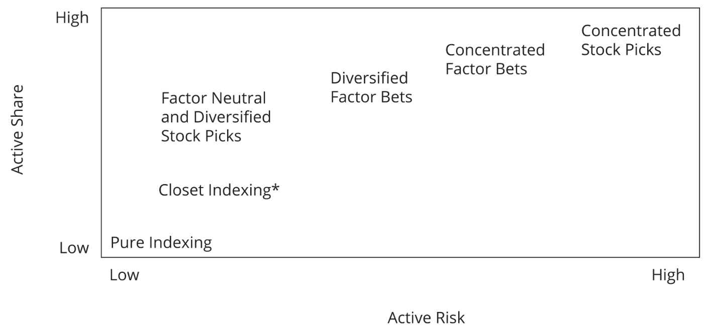
• A closet indexer is defined as a fund that advertises itself as being actively managed but is substantially similar to an index fund in its exposures
• A sector rotator would need to have large permitted deviations in sector weights
• A stock picker would need to have large permitted deviations in individual security weights
• A diversified multi-factor investor has large sector deviations and limited single-security deviation, and low tracking error

Chapter: Derivative and Currency Management

Option Strategy

Covered Call

Protective Put

Collar

Straddle

Bull Spread and Bear Spread

Calendar Spread

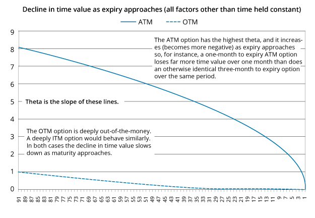
Options that are close to ATM have the highest thetas, and these increase as expiration approaches. In other words ATM options lose time value at an increasing rate as they mature.

calendar spreads exploit the difference in theta between close-to-expiry and more-distant-from-expiry options. For options that are near to ATM, the nearer-dated options will have a higher absolute value of theta (more negative) than longer-dated options.

A long calendar spread: buying longer-dated options and selling shorter-dated options with the same strike and underlying. In principle the premium on the shorter-dated should fall faster than the premium on the longer-dated. Thus more value is gained on the short position than is lost on the long position, and a net profit is realized. The options need to be close to ATM, and little movement should be anticipated in the underlying over the period to expiry of the nearer-dated option (large movement might undermine the profit from the strategy). Both options will either be calls or puts, and the choice between calls and puts will reflect the investor’s view on the longer-term prospects for the stock (calls if bullish, puts if bearish).

A short calendar spread: selling longer-dated options and buying shorter-dated options with the same strike and underlying. When options are sufficiently ITM or OTM the thetas are relatively higher for the longer-dated options. the belief is that the longer-dated options will lose time value relatively more rapidly, thus the position as a whole should gain. The short calendar spread strategy is vulnerable, however, to the underlying moving so the options end up ATM when the shorter-dated option expires (so the longer-dated option premiums rise, unless implied volatility also falls, and overall there is a loss since we are short). If the stock moves at all during the period of the strategy, it would be better for it to move a lot.

In general:

• A long calendar spread will benefit from a stable market or an increase in implied volatility.
• A short calendar spread will benefit from a big move in the underlying market or a decrease in implied volatility.

Risk reversal

volatility skew, is where implied volatility increases for more OTM puts, and decreases for more OTM calls. This is explained by OTM puts being desirable as insurance against market declines (so their values are bid up by higher demand, and higher values imply higher volatility), while the demand for OTM calls is low.

If a trader believes that put implied volatility is relatively too high, compared to that for calls, a long risk reversal could be created by buying the OTM call (seen as relatively underpriced) and selling the OTM put (seen as relatively overpriced) for the same expiration.

The net positive delta exposure is then hedged by shorting the underlying stock.

BPVHR

BPVHR, i.e. Basis Point Value Hedge Ratio

$$\begin{aligned} \text{BPVHR} & = \frac{\text{BPV}_{\text{target}} - \text{BPV}_{\text{port}}}{\text{BPV}_{\text{futures}}} \\ & = \frac{\text{BPV}_{\text{target}} - \text{BPV}_{\text{port}}}{\text{BPV}_{\text{CTD}}} \times \text{CF} \end{aligned}$$

where:

• $\text{BPV}_{\text{CTD}}$ = $\text{MD}_{\text{CTD}} \times 0.0001 \times [\text{price} / 100 \times \text{contract size}]$
• $\text{BPV}_{\text{futures}} \approx \frac{\text{BPV}_{\text{CTD}}}{\text{CF}_{\text{CTD}}}$
• CF: conversion factor

FOMC % probability of rate change

FOMC, i.e. The Federal Open Market Committee

$$\frac{ \text{effective rate implied by future} - \text{current fed target rate} }{ \text{fed fund rate assuming change} - \text{current fed target rate} }$$

Cross-Currency Basis & Swap

Cross-Currency Basis represents the additional cost of borrowing dollars synthetically with a currency swap relative to the cost of borrowing directly in the USD cash market. Typically, when describing basis we view it from the foreign-currency perspective rather than the USD perspective. If the cost of borrowing dollars synthetically via a swap is greater than the cost of direct USD borrowing, the foreign currency is said to be exhibiting negative basis. Most currencies have shown a negative basis against the dollar since the financial crisis of 2008. The implication is that the USD borrower must accept a lower interest rate on the foreign-currency interest payments it receives.

currency swap only exchanges interest payments. But cross-currency basis swap exchanges both interest and notional principal of each currency at the beginning and end of the swap. Typically, the periodic payments are floating for floating.

Rationale:
A foreign company requiring USD, might not have access to direct USD borrowing or finds it prohibitively expensive.

e.g.:
A French company requires $50 million to invest in US. The cost to borrow USD directly is MRR + 100 bp. it decided to borrow for 4 years in euros at Euribor + 60 bp with interest paid quarterly, and enter a currency swap to exchange euros for dollars. Basis on the Eurodollar swap is being quoted at –20 bps. The swap pays variable interest on both legs on a quarterly settlement basis. The current $/€ exchange rate is $1.1815.

The three-month euro reference rate is 1.5% and U.S. dollar reference rate is 2.0% at swap initiation. Three months later at the first settlement date, the three-month euro reference rate is 1.6% and the U.S. dollar reference rate is 1.9%.

• At initiation

Principal flows: $50,000,000 / $1.1815 = €42,319,086

the company borrows €42,319,086 and exchange it for $50,000,000. These amounts will be swapped back at maturity.

• At first settlement

Pays:

• € interest on the loan: €42,319,086 × (0.015 + 0.006) × 90 / 360 = €222,175
• $ interest on the swap: $50,000,000 × 0.02 × 90 / 360 = $250,000

Receives:

• € interest on the swap: €42,319,086 × (0.015 − 0.002) × 90 / 360 = €137,537

Cost of $ financing:

• Cost of borrowing $ direct: $50,000,000 × (0.02 + 0.01) × 90 / 360 = $375,000 (U.S. dollar reference rate + 100 bp)

• Cost of synthetic $ borrowing: $50,000,000 × (0.02 + 0.006 + 0.002) × 90 / 360 = $350,000 (U.S. dollar reference rate + 80 bp)

• Net benefit of swap: $375,000 − $350,000 = $25,000

• Net benefit of swap: $50,000,000 (1% − 0.8%) × 90 / 360 = $25,000

• At second settlement

Pays:

• € interest on the loan: €42,319,086 × (0.016 + 0.006) × 90 / 360 = €232,755
• $ interest on the swap: $50,000,000 × 0.019 × 90 / 360 = $237,500

Receives:

• € interest on the swap: €42,319,086 × (0.016 − 0.002) × 90 / 360 = €148,117

Cost of $ financing:

• Cost of borrowing $ direct: $50,000,000 × (0.019 + 0.01) × 90 / 360 = $362,500 (U.S. dollar reference rate + 100 bp)
• Cost of synthetic $ borrowing: $50,000,000 × (0.019 + 0.006 + 0.002) × 90 / 360 = $337,500 (U.S. dollar reference rate + 80 bp)
• Net benefit of swap: $362,500 − $337,500 = $25,000
• Net benefit of swap: $50,000,000 (1% − 0.8%) × 90 / 360 = $25,000

note:

• same principal amounts are exchanged at maturity as initialization. (i.e. no exchange risk on principal)
• the European company is the dollar payer; the swap dealer is the euro payer.
• By borrowing in euros and entering a currency swap, the company has locked into a cost of the U.S. dollar reference rate + 80 bp for their USD borrowing, reflecting the 60 bp spread above the euro reference rate on the loan and the –20 bp on the swap.

VIX

CBOE Volatility Index, i.e. VIX, measures implied volatility in the S&P 500 Index over a forward period of 30 days. VIX computes a weighted average of implied volatility inferred from S&P 500 traded options (calls and puts) with an average expiration of 30 days. The VIX Index value is the annualized standard deviation of the expected +/− percentage moves in the S&P 500 Index over the following 30 days.

e.g. if the VIX was at 20, we could interpret it as telling us that the market expects that the S&P will stay within a +/−20% range over one year with a 68% level of confidence. This implies a range +/− $\frac{20}{\sqrt{12}} = 5.77\%$ over the next 30-day period.

VIX futures

The VIX futures price can be interpreted as the expected S&P 500 Index volatility in the 30-day period after the futures contract expiration date. An equity holding can be protected from extreme downturns (tail risk) by buying VIX futures. Selling VIX futures creates a short volatility position and captures the volatility risk premium embedded in S&P 500 options. Short volatility positions can result in large losses if expected volatility rises significantly. The term structure of VIX futures can provide insights into the market’s expectations of volatility over time.

VIX Options

VIX options are cash-settled European-style options. VIX options can only be exercised at contract maturity; therefore, the value of the option is determined by the expectations of VIX at the contract expiry.

Other volatility Indexes

Volatility indexes also exist on European stock market indexes. Using similar methodology to the VIX Index, VSTOXX is an implied volatility-based index based on the EURO STOXX 50 Index. VFTSE is a volatility index based on the FTSE 100, and VDAX-NEW is based on the DAX 30.

Variance Swaps

The party receiving the variable payment (the purchaser) will gain on the contract when the realized variance is greater than the implied variance and will lose when the realized variance is less than the implied variance. A variance swap can, therefore, be viewed as a pure play on whether realized variance will be higher or lower than expected variance (implied variance) over the tenor of the swap.

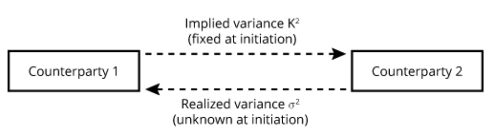
There is no exchange of notional principal at the initiation of the swap. A variance swap also has no interim settlement periods. With a variance swap, there is a single payment at the expiration of the swap based on the difference between actual and implied variance over the life of the swap:

$$\text{settlement amount}_T = (\text{variance notional})(\text{realized variance} - \text{variance strike})$$

The value of the swap is zero at initiation because implied volatility is the best ex ante estimate of realized volatility.

Realized variance is calculated by taking the natural log of the daily price relatives, the closing price on day t, divided by the closing price on day t − 1:

$$R_i = ln(P_t / P_{t-1})$$

If having N days of traded prices, we can compute N − 1 price relatives ®:

$$\text{daily variance} = \sum_{i=1}^{N-1} \frac{R_i^2}{(N-1)}$$

annualized variance = daily variance × 252

The notional amount for a variance swap can be expressed as either variance notional ($N_{var}$) or vega notional ($N_{vega}$).

$$\begin{aligned} pnl &= N_{\text{var}} \times (\sigma^2 - K^2) \\ &= N_{\text{vega}} \times (\frac{\sigma^2 -K^2}{2K}) \end{aligned}$$

since:

$$\text{variance notional} = \frac{\text{vega notional}}{2 \times \text{strike price (K)}}$$

Currency Quotes

The Price and Base Currencies: The base currency is the denominator of the exchange rate and it is priced in terms of the numerator. Unless clearly identified otherwise, the terms “buy” and “sell” refer to the base currency. e.g. sell spot 1,000,000 at CAD/USD 0.9800 is assumed to mean sell for “immediate delivery” 1,000,000 U.S. dollars and buy 980,000 Canadian dollars.

Bid/Asked Rules: Currencies are quoted with a bid/offered or bid/asked price. By convention, the smaller number is written first and the larger number is second. e.g. A quote of 0.9790/0.9810 CAD/USD. The customer pays the bid/ask spread, paying more and/or receiving less in the transaction.

Forward points are an adjustment to the spot price to determine the forward price, e.g.

Spot Quote	Forward Points	Points with Decimal Adjusted	Forward Price
1.33	1.1	1.1 / 100 = 0.011	1.33 + 0.011 = 1.341
2.554	–9.6	–9.6 / 1,000 = –0.0096	2.554 − 0.0096 = 2.5444
0.7654	13.67	13.67 / 10,000 = 0.001367	0.7654 + 0.001367 = 0.766767

Spot and forward bid/asked, e.g.

Maturity/Settlement	Spot Quote/Forward Points
Spot AUD/EUR	1.2571/1.2574
30 days	–1.0/–0.9
90 days	+11.7/+12.0

FX Swap, a misnomer, rolls over a maturing forward contract using a spot transaction into a new forward contract. An existing forward is “swapped” for another forward transaction.

Currency effects on return and risk

return

$$\begin{aligned} R_{DC} &= (1+R_{FC})(1+R_{FX}) - 1 \\ &\approx R_{FC} + R_{FX} \end{aligned}$$

note:

• $R_{DC}$ = asset return denoted in domestic currency
• $R_{FC}$ = asset return denoted in foreign currency
• $R_{FX}$ = percentage change in value of the foreign currency denoted in D/F (use domestic/foreign and then solve as EV / BV − 1 = $R_{FX}$)

risk

$$\sigma_{R_{DC}}^2 \approx \sigma_{R_{FC}}^2 + \sigma_{R_{FX}}^2 + 2\sigma_{R_{FC}}\sigma_{R_{FX}}\rho_{(R_{FC}, R_{FX})}$$

note:

• for domestic investor, $\sigma_{R_{DC}}^2$ is usually higher than $\sigma_{R_{FC}}^2$, meaning more risk
• correlation between $R_{FC}$ and $R_{FX}$ matters:
  • if positive, $R_{FC}$ is amplified by $R_{FX}$, increasing the volatility to domestic investor
  • if negative, $R_{FC}$ is dampened by $R_{FX}$, decreasing the volatility to domestic investor

special case if $R_{FC}$ is a risk-free return:

$$\sigma{R_{DC}} = \sigma_{R_{FX}} (1 + R_{FC})$$

minimum variance hedge ratio (MVHR) is a mathematical approach to determining the hedge ratio. When applied to currency hedging, it is a regression of the past changes in value of the portfolio $R_{DC}$ to the past changes in value of the $R_{FX}$ to minimize the variance of $R_{DC}$. The hedge ratio is the beta (slope coefficient) of that regression. e.g.

$R_{DC}$ = 0.12 + 1.25(%Δ$S_{USD/EUR}$) + ε

hedge ratio = 1.25, the manager will short EUR 1.25 times a long EUR exposure in the portfolio

NDFs

NDFs, i.e. Non-Deliverable Forward, alternative to deliverable forwards and require a cash settlement of gains or losses in a developed market currency at settlement rather than a currency exchange. Emerging market governments frequently restrict movement of their currency into or out of the country to settle normal derivative transactions. Such countries have included Brazil (BRL), China (CNY), and Russia (RUB).

A benefit of NDFs is lower credit risk because delivery of the notional amounts of both currencies is not required. Only the gains to one party are paid at settlement, made in the developed market currency.

Chapter: Alternative Investment

Hedge Fund Strategy

six strategy categories:

• 1. Equity related
• 2. Event driven
• 3. Relative value
• 4. Opportunistic
• 5. Specialist
• 6. Multi-manager

Equity-related

Ranked by overall long exposure to market

L/S Equity:

L/S Equity, i.e. Long/Short Equity. The fund manager longs stocks that they think will rise, and shorts stocks that they believe will fall.

• typically have 40% - 60% net long exposure, benefitting from market’s long term upward trend
• more concentrated on particular sector or industry
• aspire to provide returns comparable to long-only fund, but with half of volatility
• may use leverage to achieve worthwhile returns

Example:

• Long extension: net exposure of 100%. e.g. 130/30 fund (gross exposure 160%)

EMN:

EMN, i.e. Equity Market Neutral

• near-zero market risk exposure; (immune to overall market movements)
• systematic approach to take long and short positions in diversified stocks
• alpha seeking, low volatility
• leverage is generally applied to achieve acceptable level of return

Dedicated Short Selling and Short-Biased

dedicated short-selling: pure shorts overpriced stocks (e.g. poorly managed, in declining market segment, or with deceitful accounting); typically 60% - 120% short (by holding the rest in cash).

short-biased, similar except somewhat offset by a long exposure

• negative corr with market, lower returns, greater volatility, little leverage
• activist short selling: not only shorts, but also presents research that contends overprice

Event driven

• soft-catalyst event-driven approach: investment made before an event is being announced
• hard-catalyst event-driven approach: investment made after a corporate event is being announced, taking advantage of security prices that have not fully adjusted.

note: Soft-catalyst investing is generally more volatile and, thus, riskier than a hard-catalyst approach.

Merger Arbitrage

long target company stock, and short acquiring company stock. Reverse if assume a failed merger (e.g., antitrust regulation)

• possibly 300% to 500% leverage for returns
• high sharpe ratios (relatively steady returns), but large left-tail risk (merger unexpectedly fails)

Distressed Securities

take positions in the securities of firms that are in financial distress, including firms that are in bankruptcy or near bankruptcy. Firms may find themselves in this position for a number of reasons, including too much leverage, difficulty competing in their sector, or accounting issues. The securities of such a firm will often trade at greatly depressed prices.

Compounding the discounting of the securities of distressed firms is the fact that institutions such as insurance companies and banks are often not permitted to hold non-investment-grade securities. The selling of such securities can create significant pricing inefficiencies and can open up opportunities for hedge funds seeking profit.

Relative Value

attempt to exploit valuation differences between securities

Fixed-Income Arbitrage

take advantage of temporary mispricing of fixed-income instruments, by going long comparatively undervalued securities, and going short comparatively overvalued securities, under the assumption that prices will revert toward their fair values.

• Yield curve trades: anticipated changes in yields
• Carry trades: long high-yielding and short low yielding

note:

• substantial leverage is often applied, since fixed-income securities tend to be priced fairly efficiently, the amount of profit that can be earned by fixed-income arbitrage is somewhat limited. 400% leverage is not uncommon; even 1500% leverage is not unheard of.

Convertible Bond Arbitrage

One way to view convertible bonds is as a regular bond plus a long call option on the corresponding stock

exploit the fact that the options within convertible instruments usually exhibit low implied volatilities when compared to the historical volatilities of the equities that underlie the option. To do this without taking on excess risk, convertible bond arbitrageurs will take on other positions to try to hedge out the delta and gamma risk of the convertible bond holdings.

buy relatively undervalued convertible bond and short the relatively overvalued underlying stock

• delta-hedge based on delta of the convertible bond, typically 300% long vs 200% short
• profitable if realized equity volatility exceeds implied volatility of convertible’s embedded option net of costs.

Opportunistic

top-down focus on regions, sectors, asset classes (not individual securities). Diversification potential with traditional assets, often with beneficial right-tail skew. Highly liquid, and high leverage.

Global Macro

identify global economic changes (e.g. inflation, FX, rates). may use significant leverage (600% - 700%). Can have high alpha and strong diversification potential. Successful manager being contrarian, investing ahead of others.

Managed Futures

invest long-short via derivatives, usually with high leverage (built-in feature of margin trading). Possible crowding. Typically systematic. many based on volatility or momentum. use signals for exit.

Specialist

Volatility trading

exploit mispriced volatility (exploit skew and smile volatility surface), using:

• options (e.g. straddles, calendar and price spreads)
• futures on VIX
• Variance swaps

note:

• potential large gains due to convexity of volatility derivatives
• hard to benchmark

Reinsurance / Life settlements

• Life settlement: HF buys policy from insured, takes over premium payments and receives death benefits

• Catastrophe risk reinsurance: HF buys earthquake, tornado, hurricane, flood, etc insurance from reinsurer. Considerable expertise required. Typically illiquid.

Multi-manager

A portfolio of various HF diversified strategies

FoF (Funds-of-funds)

typically 2% management fees + 20% performance incentive on gross gains net of management fees & expenses. Plus fees charged by FoF manager. Lack of transparency into individual HFs; principle-agent issues. Multi-layer fees, no performance fee netting across managers. May include HFs otherwise inaccessible.

Multi-strategy funds

One org, better knowledge over when, how much capital and leverage, of fund correlations and risks. Ease of reallocation between strategies. Absorb netting risk internally (favorable fees). Less diversified operational risk.

Investment Opportunity Set

• traditional approach:

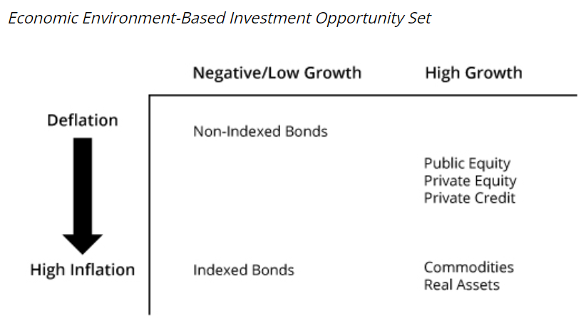
• risk factor based approach:

defining asset classes by statistically estimating their sensitivities to risk factors, e.g. economic growth and inflation, interest rates and credit spreads, or currency values, liquidity, capitalization, and value-versus-growth.

advantage:

• Identifying sources of risk that are common across asset classes, mitigating a limitation of the traditional approaches, which may classify investments into different classes even when they face largely the same risk factors, leading a manager to believe the portfolio is more diversified than it actually is.
• by allowing a manager to analyze multiple dimensions of portfolio risk, this approach is useful for developing an integrated risk management framework. In this sense, it can be more useful than the traditional approaches for highlighting the primary drivers of portfolio risk.

disadvantage:

• risk factor estimates can be sensitive to the period used for analysis
• The results may also be more difficult to communicate to decision makers and to implement compared to traditional approaches.

Chapter: Private Wealth Management

TTLLU-RR

set of consideration for private wealth management

• T: Time horizon;
• T: Taxes;
• L: Liquidity
• L: Legal issues
• U: Unique Constraints
• R: Returns
• R: Risk
  • ATBR: ability to bear risk
  • WTBR: willingness to bear risk

SAMURAI

criteria for a good benchmark

• S: Specified in advance
• A: Appropriate and consistent with the manager’s investment style
• M: Measurable
• U: Unambiguous, able to clearly identify the securities
• R: Reflective of current investment opinions
• A: Accountable, accepted by the manager
• I: Investible, possible to replicate passively

Portfolio Reporting

Portfolio reporting enables private clients to understand how their investment portfolio is performing and whether their financial goals are likely to be achieved. It provides a basis for a private wealth manager to review a client’s IPS and investment strategy with the client to determine if changes are required to achieve the client’s goals.

• Performance summary for the current period.
• Market commentary for the current period to provide context for the portfolio’s performance.
• Portfolio asset allocation at the end of the current period, including strategic asset allocation - weights or tactical asset class target ranges.
• Detailed performance of asset classes and individual securities.
• Benchmark report comparing asset class and overall portfolio performance to appropriate benchmarks.
• Historical performance of client’s investment portfolio since inception.
• Transaction details for the current period (e.g., contributions, withdrawals, interest, dividends, and capital appreciation).
• Purchase and sale report for the current period.
• Impact of currency exposure and exchange-rate fluctuations.
• Progress toward meeting goal portfolios when using a goals-based investing approach.

Portfolio Review

A portfolio review enables the private wealth manager to reassess a client’s IPS and investment strategy in light of recent performance to determine if changes are required. A portfolio review typically addresses the following areas:

• Appropriateness of client’s existing goals and investment parameters and if any changes are required.
• Rebalancing of portfolio asset allocation to target allocation or ranges.
• Any changes to the wealth manager’s ongoing management of the portfolio (e.g., degree of - discretionary authority).
• Any changes or updates in the wealth manager’s duties and responsibilities.
• Any changes to IPS and portfolio review frequency.

Balance Sheet Management of Banks and Insurers

how changes in the market value of assets, liabilities, and leverage levels affect the change in the market value of equity is:

$$\%\Delta E = \%\Delta A \cdot M - \%\Delta L \cdot (M - 1)$$

where:

• $\%\Delta E$ = percentage change in the value of equity
• $\%\Delta A$ = percentage change in the value of assets
• $\%\Delta L$ = percentage change in the value of liabilities
• M = leverage multiplier, A / E

The sensitivity of the institution’s equity capital to a unit change in the reference yield, y, of the assets (i.e., the modified duration of the equity capital) is:

$$D_E = D_A \cdot M - D_L \cdot (M - 1) \cdot \frac{\Delta i}{\Delta y}$$

where:

• $D_E$ = modified duration of the institution’s equity capital
• $D_A$ = modified duration of the institution’s assets
• $D_L$ = modified duration of the institution’s liabilities
• M = leverage multiplier, A / E
• $\frac{\Delta i}{\Delta y}$ = estimated change in yield of liabilities, i, relative to a unit change in yield of assets, y

Expected volatility of the percentage changes in the market value of equity capital:

$$\sigma_E^2 = M^2 \sigma_A^2 + (M - 1)^2 \sigma_L^2 - 2 M (M - 1) \sigma_A \sigma_L \rho_{AL}$$

where:

• $\sigma_E$ = standard deviation of percentage change in the market value of equity
• $\sigma_A$ = standard deviation of percentage change in the value of assets
• $\sigma_L$ = standard deviation of percentage change in the value of liabilities
• M = leverage multiplier, A / E
• $\rho_{AL}$ = correlation of percentage value changes in assets and liabilities

Estate Planing

Lifetime Gifts vs Testamentary Bequests:

$$\begin{aligned} & FV_{\text{gift}} &&= [1 + r_g(1-t_g)]^n(1-T_g) \\ & FV_{\text{bequest}} &&= [1 + r_e(1-t_e)]^n(1-T_e) \\ & RV &&= \frac{FV_{\text{gift}}}{FV_{\text{bequest}}} \end{aligned}$$

note:

• RV of tax-free gift, $T_g = 0$

Life Insurance cost comparison

• Net payment cost index: assumes the individual dies at the end of the horizon and cash value is not considered
• Net surrender cost index: assumes the individual terminates the policy (insurance ceases) at the end of the horizon and the cash value is received

steps:

• 1. use annuity due (BGN mode) to compute FV of the premium
• 2. use ordinary annuity (END mode) to compute FV of the dividend
• 3. $FV_{\text{premium}} - FV_{\text{dividend}}$, further minus cash value if using new surrender cost index
• 4. use annuity due (BGN mode) to compute annuitized cost

Growth-adjusted discount rate

$$r = (1 + r) / (1 + g) - 1$$

Taxation

After-Tax Holding Period Return

$$R' = \frac{value_1 - value_0 + income - tax}{value_0}$$

or

$$R' = R - \frac{tax}{value_0}$$

note:

• if any intermediate cashflow paid as income, adjust $value_0$ using the way used in modified dietz return

After-Tax Post-Liquidation Return

$$R_{PL} = \sqrt[n]{(1 + R'_1)(1 + R'_2) \cdots (1 + R'_n)(1 - \text{liquidity tax} / {\text{final value}})} - 1$$

After-Tax Excess Return

$$x' = R' - B'$$

where:

• $R'$ = after-tax return of the portfolio
• $B'$ = after-tax return of the benchmark

$$\alpha_{\text{tax}} = x' - x$$

where:

• $x'$ = after-tax excess return
• $x$ = pretax excess return

Tax-Efficiency Ratio (TER)

$$TER = \frac{R'}{R}$$

where:

• $R'$ = after-tax return
• $R$ = pretax return

note:

• for positive returns in taxable accounts, the higher the TER, the better.

Chapter: Trading, Performance Evaluation

Implementation Shortfall

IS (i.e. implementation shortfall) measures the total cost of trading, expressed as basis points of the total cost of the paper portfolio. e.g. buy order

$$\text{IS} = \text{paper return} - \text{actual return}$$

where:

• $\text{paper return} = \text{total order size} \times (\text{close price} - \text{decision price})$
• $\text{actual return} = \text{filled order size} \times (\text{close price} - \text{execution price}) - \text{commission}$

Decomposition of IS. e.g. buy order

• Execution cost = $\text{filled order size} \times (\text{execution price} - \text{decision price})$
  • Delay cost = $\text{filled order size} \times (\text{arrival price} - \text{decision price})$:
  • trading cost (i.e. market impact cost) = $\text{filled order size} \times (\text{execution price} - \text{arrival price})$
• Opportunity cost = $\text{unfilled order size} \times (\text{close price} - \text{decision price})$
• Fixed cost = $\text{filled order size} \times \text{commission}$

note:

• for sell order, flip the sign
• execution risk: adverse price movement occurs over the trading horizon (in volatile market)
• market impact cost: trade at more adverse prices to execute a larger transaction (in illiquid market)

Market-adjusted cost

market-adjusted cost removes the impact of market movements on trade cost.

$$\text{market-adjusted cost} \text{(bps)} = \text{arrival cost} \text{(bps)} - \beta \times\text{index cost} \text{(bps)}$$

where:

• arrival cost = $\text{side} \times (\text{execution price} / \text{arrival price} - 1)$
• index cost = $\text{side} \times (\text{index average price} / \text{index arrival price} - 1)$

Return Attribution

$$R_A = \sum\limits_{i=1}^N{\Delta W_i}{R_i}$$

where:

• $R_i$: return from security i
• $\Delta W_i$: active weight of security i, i.e. diff between portfolio and benchmark weight

BHB Method, i.e. Brinson-Hood-Beebower

$$\begin{aligned} \text{Portfolio Return}, R = \sum\limits_{i=1}^n{w_i}{R_i} \\ \text{Benchmark Return}, B = \sum\limits_{i=1}^n{W_i}{B_i} \end{aligned}$$

where:

• $w_i$: portfolio weight of the ith segment (e.g. style, sector, geography, etc.)
• $R_i$: portfolio return in the ith segment
• $W_i$: benchmark weight of the ith segment
• $B_i$: benchmark return in the ith segment
• n: number of segments

$$\begin{aligned} R_A & = R - B \\ & = \sum\limits_{i=1}^n{w_i}{R_i} - \sum\limits_{i=1}^n{W_i}{B_i} \\ & = \sum\limits_{i=1}^n(w_i R_i - W_i B_i) \\ & = \sum\limits_{i=1}^n[\underbrace{(w_i - W_i)\cdot B_i}_{\text{Allocation Effect}} + \underbrace{Wi \cdot (R_i - B_i)}_{\text{Selection Effect}} + \underbrace{(w_i - W_i) \cdot (R_i - B_i)}_{\text{Interaction Effect }}] \end{aligned}$$

BF Method, i.e. Brinson-Fachler

to solve BHB Method’s issue of misleading allocation effect, due to the sign of the resulting allocation effect does not automatically indicate whether the decision to overweight/underweight a particular segment of the portfolio was correct.

$$\text{Allocation Effect} = (w_i - W_i)\cdot (B_i - \bm{B})$$

where:

• B: overall benchmark return

note:

• the additional term: $\sum\limits_{i=1}^n(w_i - W_i) \cdot (-B) = (\sum\limits_{i=1}^n{w_i} - \sum\limits_{i=1}^n{W_i}) \cdot (-B) = (1 - 1) \cdot (-B) = 0$

Arithmetic vs Geometric Attribution

	Period 1	Period 2
Portfolio Return ®	5%	5%
Benchmark Return (B)	3%	3%

• arithmetic attribution: $R_A = R - B = 5\% - 3\% = 2\%$
• geometric attribution: $R_A = \frac{1 + R}{1 + B} - 1 = \frac{1.05}{1.03} - 1 = 1.94\%$

geometric attribution does compound across periods: $(1 + 1.94\%)^2 - 1 = (1.05/1.03)^2 - 1 = 3.92\%$

Performance Metrics

Sharpe Ratio

calculated as excess return over the risk-free rate (numerator) divided by standard deviation (denominator)

$$S_A = \frac{\bar{R}_A - \bar{r}_f}{\hat{\sigma}_A}$$

note:

• denominator does not differentiate between volatility that is upside versus downside. Therefore, there is a penalty for all volatility, even if it is “good” volatility (addressed in Sortino Ratio below).

Treynor Ratio

similar to the Sharpe ratio, but the denominator is measured by beta, so only considering systematic risk rather than total risk

$$T_A = \frac{\bar{R}_A - \bar{r}_f}{\hat{\beta}_A}$$

note:

• assume efficient markets
• only useful in evaluating portfolios that have systematic risk and do not have unsystematic risk (i.e. well diversified)

Information Ratio

measures a portfolio’s performance against the benchmark but accounts for differences in risk

$$IR = \frac{E(r_p) - E(r_B)}{\sigma(r_p - r_B)}$$

note:

• the denominator is known as the tracking risk, or the variability in the portfolio performance with that of its benchmark

Appraisal Ratio

measures the ratio of active return, α, to the volatility of the residual term, $σ_ε$, both derived from a factor-based regression

$$AR = \frac{α}{σ_ε}$$

note:

• higher AR indicates generating more active return per unit of active risk (as represented by residual risk $σ_ε$ also referred to as the “standard error of the regression”) and is therefore a superior active manager according to this measure.
• $σ_ε$, i.e. the standard error of the regression, is the volatility of the error term in a factor-based regression, representing the component of the volatility of returns not explained by the regression model factors. This component of volatility is generated by the manager taking active bets relative to the factors in the model, hence $σ_ε$ here is playing the role of active risk.
• The AR is analogous to the IR. It looks at active return per unit of active risk. The only difference is that the AR uses a factor-based regression to estimate active return and active risk.

Sortino Ratio

only considers the standard deviation of the downside risk, in contrast to the Sharpe ratio, which considers all risk (e.g., both upside and downside). Positive volatility associated with the upside can be considered “good” volatility. As a result, the Sortino ratio can provide a more meaningful view of a portfolio’s risk-adjusted performance than the Sharpe ratio.

$$SR_D = \frac{E(r_p) - r_T}{\sigma_D}$$

where:

• $r_T$: target rate of return, or minimum acceptable return (MAR)
• $\sigma_D$: target semideviation, measuring the standard deviation of returns below the target return

note:

• determination of MAR is subjective and specific to each investor, causing comparability problems

Capture Ratio

Capture Ratio (CR) = UC ratio / DC ratio, a measure of return asymmetry, > 1 = positive asymmetry (convex shape), < 1 = negative asymmetry (concave shape)

$$\text{Capture Ratio} = \frac{\text{Upside Capture Ratio}}{\text{Downside Capture Ratio}}$$

e.g.

• if portfolio return is 5%, and benchmark return is 4%, then upside capture ratio 5% / 4% = 125%, > 100% indicates outperformed
• if portfolio return is -3%, and benchmark return is -4%, then downside capture ratio -3% / -4% = 75% < 100% indicates outperformed
• then the capture ratio is 125% / 75% = 1.67, indicates a positively asymmetrical (convex) return profile

note:

• ideally, the manager would capture as much of the upside as possible and capture as little of the downside as possible to maximize the capture ratio
• when betas are increasing (decreasing), momentum-driven strategies should have higher (lower) UC than value-driven strategies. A low-beta (high-beta) strategy will have lower (higher) UC and DC. Therefore, CRs can be used to confirm the investment strategy.

Drawdown

Month	Monthly Return	Drawdown	Cumulative Drawdown	Comments
01/2018	3.14%		0.00%
02/2018	–2.55%	–2.55%	–2.55%	Drawdown phase begins
03/2018	–2.71%	–2.71%	–5.26%
04/2018	–4.66%	–4.66%	–9.92%
05/2018	–4.91%	–4.91%	–14.83%
06/2018	–0.73%	–0.73%	–15.56%	Maximum drawdown
07/2018	2.18%		–13.38%	Recovery phase begins
08/2018	3.11%		–10.27%
09/2018	2.45%		–7.82%
10/2018	3.65%		–4.17%
11/2018	4.03%		–0.14%
12/2018	4.14%		0.00%	Drawdown recovered

Time-to-Cash Table

liquidity classification schedule (time-to-cash table) is used to manage liquidity risk, including:

• 1. amount of time needed to convert assets to cash
• 2. liquidity classification level
• 3. liquidity budget

Time to Cash	Liquidity Classification	Liquidity Budget (% of portfolio)
< 1 week	Highly liquid	At least 5%
< 1 quarter	Liquid	At least 25%
< 1 year	Semi-liquid	At least 40%
> 1 year	Illiquid	Up to 40%

Ethical and Professional Standards

GIPS return calculation

Rt to be evaluated each time an interim ECF occurs. Then sub-periods returns are geometrically linked to create a TWRR (i.e. time-weighted rate of return).

$$R_t = \frac{EV - BV}{BV}$$

$$R_{TWRR} = (1+R_1) \times (1+R_2) \times \cdots \times (1+R_t)$$

Approximations when portfolios are not valued daily, and ECFs (i.e. external cash flows) are relatively small. The larger the ECFs and the more volatile the market, the greater the discrepancy will be between the true TWRR and the approximations.

Modified Dietz Return

$$R_{MD} = \frac{EV - BV - ECF}{BV + \text{adjusted ECF}}$$

$$\text{adjusted ECF} = \sum{\text{ECF} \times \text{weight}}$$

where:

• weight is based on proportion of days in use, e.g. if the 1st ECF was received on Day 7, meaning that the manager had use of it for 23 days. Then the weight is 23/30.

note:

• ECFs will be positive if cash inflow, and negative if cash outflow

MIRR

MIRR (i.e. modified internal rate of return)

$$EV = BV(1+r) + \sum{ECF(1 + r)^{\text{weight}}}$$

solve for r

where:

• weight is the same defined in the modified Dietz Return